Mapping the French mathematical optimization community (Part I)
Academics often rely on different metrics, such as the i10 or h-index, to determine how influential is a researcher. However, I believe these metrics say little on how close is the researcher to her affiliated community. Here, we look more closely on the coauthorship network of the optimization community in France to try to map out influential researchers and to depict the different subcommunities we could find. I believe that such analysis could prove useful for newcomers to the community and young researchers like me.
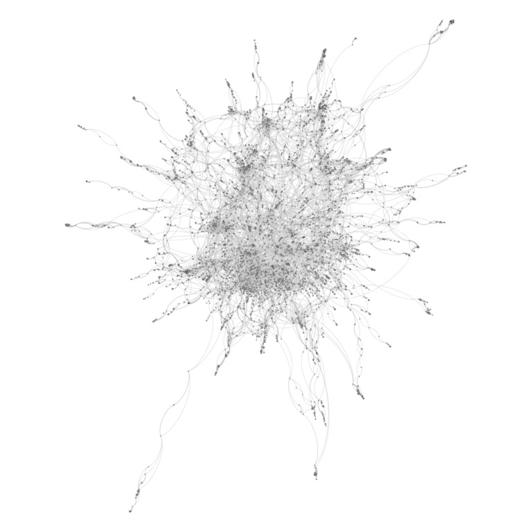
Recall that here we rely on the
coauthorship network of the French mathematical optimization community.
To do so, we have at our disposal a database of the articles published in HAL.
This database was built in a previous post, where we detailed how to parse
a bibtex file
to generate the coauthorship network with networkx. We ended up by exporting
a graph in graphml format. In this previous post, we also exhibited the limit of our
approach, which still hold true here:
- Most of the articles (79%) in our database have been published after 2010. We miss the ancient history of the community.
- We are using HAL, a service used mostly in France. We miss the collaborations with labs outside France.
- We extracted only the article published under the mathematical optimization (math-oc) tag. So our analysis will short fall when dealing with researchers disseminating their works in different communities (e.g. operation research, automatics, signal processing, machine learning...)
Having in mind these shortfalls, we would like now to push further the analysis. In the next, we show how to import the coauthorship network into LightGraphs, a graph library implemented in pure Julia. We extract the largest connected component, and derive some statistics about it. We then stress out the most central researchers in the community by using different centrality measures. We will focus on the detection of subcommunities in a future blog post.
In case, all source code is available on github.
Why using LightGraphs?
In the previous post
we started the preprocessing by using Python. So why not stick to Python
and use networkx for the remaining of our analysis?
The thing here is that networkx tends to be
slow (and I had bad experience with memory leaks occurring when analyzing
large networks). The libraries networkit and graph-tools are valid
alternatives, but come with a few caveats:
- After testing up a bit
networkit, I was a bit puzzled by the lack of documentation. Most of the time, the docstring in the C++ wrapper are missing, and I had some trouble figuring out how exactly to use the different functions. graph-toolsis impressive (really, you should check the tutorials). To the best of my knowledge, it is one of the graph libraries offering among the most advanced algorithms for community detection, based on Stochastic Block Model (SBM) analysis. However, I could not choosegraph-toolsas I am currently working on my good old personal laptop, which comes with only 4Go of RAM. Thus, I am unable to compilegraph-tool, as it requires at least 3Go of RAM and more than 1h to be compiled (I guess that's the price to depend onboost::graph).
On the contrary, LightGraphs achieves pretty good performance (as stated in this benchmark) and is a lightweight library. It is written entirely in Julia, and relying on a language with built-in linear algebra will prove useful for the next post, where we will focus on the detection of communities in our graph.
Using Julia will also allow us to use the excellent UnicodePlots library for plotting our results directly in the terminal.
Setting-up the environment
Now that we are all set, we could start our analysis.
Importing the package
We start by importing some usual packages:
using LinearAlgebra
using Statistics
and our graph library:
using LightGraphs
We will need also the following packages to load a network specified
in graphml format and the metadata from the CSV file.
# Packages to import graph from GraphML format
using EzXML
using GraphIO
# Package to handle dataframes in Julia
using DataFrames
using CSV
# For plotting
using UnicodePlots
# For printing
using Printf
Loading the coauthorship network to LightGraphs
We first load the coauthorship network into our graph library. We start by setting the path to the input graph, which should be, if we follow the naming of the previous post:
GRAPH_SRC = "coauthors.graphml"
We use GraphIO to load the graph into LightGraphs:
reader = GraphIO.GraphML.GraphMLFormat()
g = loadgraph(GRAPH_SRC, reader)
We now get a valid LightGraphs graph.
Loading the metadata
We import the metadata as a DataFrame, so we could associate to each node
of the graph a corresponding author in the community:
df = DataFrame(CSV.File("metadata.txt", delim=';', header=0))
Looking more closely at the first row, we get:
julia> df[1, :]
DataFrameRow
│ Row │ Column1   │ Column2 │ Column3                  │
│     │ String?   │ String  │ String                   │
├─────┼───────────┼─────────┼──────────────────────────┤
│ 1   │ bonnans j │ 1       │ ['Bonnans, J. Frederic'] │
I confess I forgot to specify correctly the names for each column...
The first column corresponds to the key we designed in the previous article.
The second column is the id of the corresponding node in the graph. Then,
the third column gives the associated name(s).
To get a nicer display,
we build up a function get_name which takes as input an index and returns the
corresponding author in the dataframe df.
function parse_name(name)
    regs = [r"\'(.*?)\'", r"\"(.*?)\""]
    for reg in regs
        m = match(reg, name)
        if m !== nothing
            # Remove matching ''
            return m.match[2:end-1]
        end
    end
end

function get_name(id::Int)
    # Get raw name from dataframe
    raw_name = df[id, 3]
    return parse_name(raw_name)
end
and we get:
julia> get_name(1)
"Bonnans, J. Frederic"
which is a lot more better :)
Now, we have everything set up to begin our analysis.
Splitting the community in connected components
We first focus on the connected components in the community.
Indeed, there is a little chance that the global graph g is connected.
But if we are lucky, we could extract a connected component large enough to be
meaningful for our analysis.
The global graph g has 7487 nodes and 19046 edges. Looking at it more closely,
it appears that the graph is not connected:
julia> is_connected(g)
false
Let's analyze the different connected components. We first extract
them from the original graph g:
connected_graphs = connected_components(g)
and we get 534 subgraphs ... which is large. It appears that the community is quite balkanized. Let's analyze the number of nodes in each connected components:
number_nodes = [length(s) for s in connected_graphs]
# Sort the results inplace
sort!(number_nodes, rev=true)
Looking more closely at the ten most populated subgraphs, we get
julia> number_nodes[1:10]
10-element Array{Int64,1}:
 5856
   44
   20
   19
   18
   17
   16
   16
   15
   13
So the largest subgraph has 5856 authors, whereas the second one has only 44 authors, which is less than 2 orders of magnitude lower. In fact, if we remove the largest connected component (those with 5856 authors), the remaining subgraphs have in average only 3 authors.
julia> print("Average number of nodes: ", mean(number_nodes[2:end]))
3.0600375234521575
So we could guess that almost all these micro-communities are issued by single articles.
For the remaining, we will discard all connected components except the
largest one. We build a new subgraph sg, that we will consider as the core of the
optimization community. In LightGraphs syntax, that translates to
# Get first connected component
sv = connected_components(g)[1]
sg, _ = induced_subgraph(g, sv)
The index sv allows to keep a correspondance between the indexes of the
nodes in the largest connected component sg and the nodes in the original graph
g (which themselves correspond to the index in the file metadata.txt).
From now on, the term graph and network will consist in the subgraph
sg, and we will discard the original graph g.
Looking more closely at the largest subgraph
Now that we have managed to extract the largest connected component, we could derive some statistics about it. First, we extract the number of neighbors (which is, in our case, the number of coauthors) for each author in our graph:
deg = degree(sg)
We also compute the diameter of our graph:
diam = diameter(sg)
and print out basic information about the graph sg:
println("Nodes: ", nv(sg))
println("Edges: ", ne(sg))
println("Max degree: ", maximum(deg))
println("Average degree: ", mean(deg))
println("Diameter: ", diam)
println("Density: ", density(sg))
Nodes: 5856
Edges: 16701
Max degree: 152
Average degree: 5.703893442622951
Diameter: 15
Density: 0.0009741918774761658
In plain English, that transposes to:
- We have a community with 5856 authors and 16701 coauthorships;
- The most connected author has 152 coauthors (which in my opinion is impressive, especially in math);
- Each author has in average 5.7 coauthors
- The longest distance between two authors is 15.
If we look more closely at the distribution of the number of coauthors:
histogram(deg, nbins=30, xscale=log10)
                  ┌                                        ┐
   [  0.0,   5.0) ┤▇▇▇▇▇▇▇▇▇▇▇▇▇▇▇▇▇▇▇▇▇▇▇▇▇▇▇▇▇▇▇▇▇▇ 3617
   [  5.0,  10.0) ┤▇▇▇▇▇▇▇▇▇▇▇▇▇▇▇▇▇▇▇▇▇▇▇▇▇▇▇▇▇▇ 1499
   [ 10.0,  15.0) ┤▇▇▇▇▇▇▇▇▇▇▇▇▇▇▇▇▇▇▇▇▇▇▇▇ 362
   [ 15.0,  20.0) ┤▇▇▇▇▇▇▇▇▇▇▇▇▇▇▇▇▇▇▇▇▇ 177
   [ 20.0,  25.0) ┤▇▇▇▇▇▇▇▇▇▇▇▇▇▇▇▇▇ 67
   [ 25.0,  30.0) ┤▇▇▇▇▇▇▇▇▇▇▇▇▇▇▇ 33
   [ 30.0,  35.0) ┤▇▇▇▇▇▇▇▇▇▇▇ 15
   [ 35.0,  40.0) ┤▇▇▇▇▇▇▇▇▇▇▇▇▇▇ 27
   [ 40.0,  45.0) ┤▇▇▇▇▇▇▇▇▇▇▇▇▇ 24
   [ 45.0,  50.0) ┤▇▇▇▇▇▇▇▇▇▇ 10
   [ 50.0,  55.0) ┤▇▇▇ 2
   [ 55.0,  60.0) ┤▇▇▇▇▇▇▇▇ 7
   [ 60.0,  65.0) ┤ 1
   [ 65.0,  70.0) ┤▇▇▇▇▇ 3
   [ 70.0,  75.0) ┤▇▇▇ 2
   [ 75.0,  80.0) ┤▇▇▇ 2
   [ 80.0,  85.0) ┤ 1
   [ 85.0,  90.0) ┤▇▇▇▇▇ 3
   [ 90.0,  95.0) ┤ 1
   [ 95.0, 100.0) ┤ 0
   [100.0, 105.0) ┤ 0
   [105.0, 110.0) ┤ 0
   [110.0, 115.0) ┤ 1
   [115.0, 120.0) ┤ 0
   [120.0, 125.0) ┤ 0
   [125.0, 130.0) ┤ 1
   [130.0, 135.0) ┤ 0
   [135.0, 140.0) ┤ 0
   [140.0, 145.0) ┤ 0
   [145.0, 150.0) ┤ 0
   [150.0, 155.0) ┤ 1
                  └                                        ┘
                              Frequency [log10]
We observe that 3617 authors have less than 5 coauthors, and 5116 have less than 10 coauthors (that is, 87% of the community). The distribution is heavy-tailed, with only 25 authors having more than 50 coauthors.
Degree distribution
We now display the degree distribution in our community.
deg_distrib = degree_histogram(sg)
deg_keys = keys(deg_distrib) |> collect
deg_vals = values(deg_distrib) |> collect

r = scatterplot(log10.(deg_keys), log10.(deg_vals))
xlabel!(r, "log degree")
ylabel!(r, "|nodes|")
           ┌────────────────────────────────────────┐
         4 │⠀⠀⠀⠀⠀⠀⠀⠀⠀⠀⠀⠀⠀⠀⠀⠀⠀⠀⠀⠀⠀⠀⠀⠀⠀⠀⠀⠀⠀⠀⠀⠀⠀⠀⠀⠀⠀⠀⠀⠀│
           │⠀⠀⠀⠀⠀⠀⠀⠀⠀⠀⠀⠀⠀⠀⠀⠀⠀⠀⠀⠀⠀⠀⠀⠀⠀⠀⠀⠀⠀⠀⠀⠀⠀⠀⠀⠀⠀⠀⠀⠀│
           │⠀⠀⠀⠀⠀⠀⠀⠀⠀⠀⠀⠀⠀⠀⠀⠀⠀⠀⠀⠀⠀⠀⠀⠀⠀⠀⠀⠀⠀⠀⠀⠀⠀⠀⠀⠀⠀⠀⠀⠀│
           │⠀⠀⠀⠀⠂⠀⠄⠀⠀⠀⠀⠀⠀⠀⠀⠀⠀⠀⠀⠀⠀⠀⠀⠀⠀⠀⠀⠀⠀⠀⠀⠀⠀⠀⠀⠀⠀⠀⠀⠀│
           │⡀⠀⠀⠀⠀⠀⠀⠀⠁⡀⠀⠀⠀⠀⠀⠀⠀⠀⠀⠀⠀⠀⠀⠀⠀⠀⠀⠀⠀⠀⠀⠀⠀⠀⠀⠀⠀⠀⠀⠀│
           │⠀⠀⠀⠀⠀⠀⠀⠀⠀⠀⠂⠀⠀⠀⠀⠀⠀⠀⠀⠀⠀⠀⠀⠀⠀⠀⠀⠀⠀⠀⠀⠀⠀⠀⠀⠀⠀⠀⠀⠀│
           │⠀⠀⠀⠀⠀⠀⠀⠀⠀⠀⠀⠁⢂⠀⠀⠀⠀⠀⠀⠀⠀⠀⠀⠀⠀⠀⠀⠀⠀⠀⠀⠀⠀⠀⠀⠀⠀⠀⠀⠀│
 |nodes|   │⠀⠀⠀⠀⠀⠀⠀⠀⠀⠀⠀⠀⠀⢁⠀⠀⠀⠀⠀⠀⠀⠀⠀⠀⠀⠀⠀⠀⠀⠀⠀⠀⠀⠀⠀⠀⠀⠀⠀⠀│
  (log)    │⠀⠀⠀⠀⠀⠀⠀⠀⠀⠀⠀⠀⠀⠀⠑⠀⡀⠀⠀⠀⠀⠀⠀⠀⠀⠀⠀⠀⠀⠀⠀⠀⠀⠀⠀⠀⠀⠀⠀⠀│
           │⠀⠀⠀⠀⠀⠀⠀⠀⠀⠀⠀⠀⠀⠀⠀⠒⠊⡂⠀⠀⠀⠀⠀⠀⠀⠀⠀⠀⠀⠀⠀⠀⠀⠀⠀⠀⠀⠀⠀⠀│
           │⠀⠀⠀⠀⠀⠀⠀⠀⠀⠀⠀⠀⠀⠀⠀⠀⠀⠐⡀⠀⠀⠂⠀⠀⠀⠀⠀⠀⠀⠀⠀⠀⠀⠀⠀⠀⠀⠀⠀⠀│
           │⠀⠀⠀⠀⠀⠀⠀⠀⠀⠀⠀⠀⠀⠀⠀⠀⠀⢀⢄⡂⠀⠀⠀⠀⠀⠀⠀⠀⠀⠀⠀⠀⠀⠀⠀⠀⠀⠀⠀⠀│
           │⠀⠀⠀⠀⠀⠀⠀⠀⠀⠀⠀⠀⠀⠀⠀⠀⠀⠀⠀⠐⠔⠱⠂⠀⠀⠀⠀⠀⠀⠀⠀⠀⠀⠀⠀⠀⠀⠀⠀⠀│
           │⠀⠀⠀⠀⠀⠀⠀⠀⠀⠀⠀⠀⠀⠀⠀⠀⠀⠀⠀⠉⡈⠁⣀⠁⣀⡈⠀⠀⠀⠀⠀⠀⠀⠀⠀⠀⠀⠀⠀⠀│
         0 │⠀⠀⠀⠀⠀⠀⠀⠀⠀⠀⠀⠀⠀⠀⠀⠀⠀⠀⠀⠀⡀⠀⣀⢀⡀⡀⡀⡀⡀⡀⠀⠀⠀⠀⠀⠀⠀⠀⠀⠀│
           └────────────────────────────────────────┘
           0                                        3
                          log degree
Here, we observe that the degree distribution has an asymptotic behavior when the degree \(k\) becomes large. That would tend to say that our network is Scale-free, that is, the fraction \(p(k)\) of nodes having a degree equal to \(k\) satisfies asymptotically
where \(\gamma\) is a given parameter. However, without further statistical analysis, the scale-free nature of our community remains hypothetical.
Average distance between two authors
We now aim at computing the average distance between two authors in the graph. We know that the diameter of the graph is equal to 15, so the average distance should be below this value. We use a naive algorithm, by iterating over all authors and computing their distance w.r.t. all other authors using the Bellman-Ford algorithm:
avg_distance = zeros(Float64, nv(sg))
for i in eachindex(avg_distance)
    res = bellman_ford_shortest_paths(sg, i)
    avg_distance[i] = mean(res.dists)
end
We get as average distance in our graph:
julia> mean(avg_distance)
6.244723488962793
So, the average distance is equal to 6.2. In average, we could linked any pair of two authors by using less than 7 coauthorship relations.
We are now able to compute the author at the center of the community, in the sense that his average shortest distance with other authors is the lowest.
# Get index in subgraph sg
author_min = findmin(avg_distance)[2]
# Get index in original graph g
original_index = sv[author_min]
# Extract corresponding name
name = get_name(original_index)
"Trelat, Emmanuel"
So if we follow that metric, Emmanuel Trélat is the most central author in the optimization community. This is not surprising, as Emmanuel Trélat is one of the most notorious optimization researcher in France :) However, it is legitimate to wonder if this metric is the most appropriate to determine the centrality in our graph.
Comparing different centrality measures
In fact, the notion of centrality in a graph depends a lot on the metrics used. Further, we are studying an undirected graph, and not all centrality measures generalize well to handle undirected graph. We compare here different metrics together and observe how differently they rank the authors in term of their centrality.
We try out different centrality measures, all implemented in LightGraphs:
- Closeness centrality measures the average shortest distance between an author and all other authors in the community. It is exactly the centrality we computed in the previous paragraph.
- Betweenness centrality measures the number of times an author is found inside a shortest path between two different authors.
- Degree centrality measures the connectivity of each author, in term of number of coauthors.
- Eigenvector centrality is a more complex measure, relying on concept from linear algebra. Let \(A = (a_{ij})_{ij}\) be the adjacency matrix of the graph (i.e. such that \(a_{ij} = 1\) if and only if node \(i\) and \(j\) are linked). The matrix \(A\) is real symmetric and comprises only positive values, hence the Perron-Frobenius theorem states there exists a unique largest eigenvalue \(\lambda\). Eigenvector centrality looks at one of the associated eigenvector \(x^\lambda\) (possibly normalized to ensure unicity), satisfying \(A x^\lambda = \lambda x^\lambda\). Then, the centrality of each node is set equal to \(x^\lambda_i\).
- Pagerank is a variant of eigenvector centrality, and adds a random jump assumption. Let \(N = (n_{ij})_{ij}\) be the normalized adjacency matrix (such that \(n_{ij} = 1 / deg(i)\) if node \(i\) and \(j\) are connected). Then Pagerank ranks the nodes in the graph according to the vector \(p\) satisfying \(p = \alpha N^\top p + \frac{1 - \alpha}{N}\), where we usually take \(\alpha = 0.85\).
Note that despite we start from simple algorithms to measure centrality, we end up with algorithm relying deeply on linear algebra. Connections between graph theory and linear algebra are indeed fascinating, and lay down the path to spectral graph theory.
We write up a small function to display the n most central authors
according to a centrality measure metrics.
function rank(sg::Graph, metrics, n=10)
    m = metrics(sg)
    classement = sortperm(m, rev=true)
    # From largest to lowest
    head = classement[1:n]
    @printf("* %-4s   (%7s) %-30s\n", "#", "Score", "Name")
    for i in eachindex(head)
        name = get_name(sv[head[i]])
        @printf("* %-4d * (%.1e) %-35s %s \n", i, m[head[i]], name, "*")
    end
end
As expected, we get different results if we use different centrality measures. We now look more closely at the 10 most central authors obtained with each centrality measure.
Closeness centrality
We first compute a ranking based on closeness centrality.
rank(sg, closeness_centrality)
* #      (  Score) Name
* 1    * (2.6e-01) Trelat, Emmanuel                    *
* 2    * (2.6e-01) Henrion, Didier                     *
* 3    * (2.5e-01) Lasserre, Jean-Bernard              *
* 4    * (2.4e-01) Malick, Jerome                      *
* 5    * (2.4e-01) Bonnans, J. Frederic                *
* 6    * (2.4e-01) Prieur, Christophe                  *
* 7    * (2.4e-01) Bergounioux, Maitine                *
* 8    * (2.4e-01) Ngueveu, Sandra Ulrich              *
* 9    * (2.3e-01) Delahaye, Daniel                    *
* 10   * (2.3e-01) Caillau, Jean-Baptiste              *
As before, Emmanuel Trélat is the most central author according to this measure, followed closely by Didier Henrion and Jean-Bernard Lasserre (both members of the LAAS laboratory). Then come Jérôme Malick, from Université de Grenoble, and Frédéric Bonnans, from CMAP.
Looking more closely at the results, we observe that authors closed to the authors in the center of the graph automatically get a high score, by construction. So doing a PhD with a top researcher automatically gives you a good score according to this measure.
Betweenness centrality
We now focus on the ranking given by betweenness centrality.
rank(sg, betweenness_centrality)
* #      (  Score) Name
* 1    * (1.4e-01) Trelat, Emmanuel                    *
* 2    * (9.9e-02) Henrion, Didier                     *
* 3    * (9.3e-02) Delahaye, Daniel                    *
* 4    * (7.5e-02) Lasserre, Jean-Bernard              *
* 5    * (7.4e-02) Malick, Jerome                      *
* 6    * (7.2e-02) Bonnans, J. Frederic                *
* 7    * (6.3e-02) Siarry, P. .                        *
* 8    * (4.9e-02) Mertikopoulos, Panayotis            *
* 9    * (4.6e-02) Ngueveu, Sandra Ulrich              *
* 10   * (4.5e-02) Bergounioux, Maitine                *
We get the same two first authors as before with closeness centrality, but Daniel Delahaye, from ENAC, becomes the third most connected author, in place of Jean-Bernard Lasserre.
Eigenvector centrality
If we look now at eigenvector centrality, we get a different list:
rank(sg, eigenvector_centrality)
* #      (  Score) Name
* 1    * (1.7e-01) Henrion, Didier                     *
* 2    * (1.6e-01) Lasserre, Jean-Bernard              *
* 3    * (1.6e-01) Ngueveu, Sandra Ulrich              *
* 4    * (1.6e-01) Artigues, Christian                 *
* 5    * (1.6e-01) Magron, Victor                      *
* 6    * (1.6e-01) Tanwani, Aneel                      *
* 7    * (1.6e-01) Jauberthie, Carine                  *
* 8    * (1.6e-01) Lopez, Pierre                       *
* 9    * (1.6e-01) Trave-Massuyes, Louise              *
* 10   * (1.6e-01) Joldes, Mioara                      *
Most of the authors listed here are researchers affiliated to the LAAS laboratory. It appears that the largest eigenvalue of the adjacency matrix \(A\) is "related", to some extent, to this laboratory. It would be interesting to observe the ranking we get if we look at the second largest eigenvalue, or the third one.
Pagerank
Eventually, we apply pagerank to our community network (with \(\alpha=0.85\)), and get the following results:
rank(sg, pagerank)
* #      (  Score) Name
* 1    * (3.9e-03) Delahaye, Daniel                    *
* 2    * (3.5e-03) Siarry, P. .                        *
* 3    * (2.7e-03) Bonnans, J. Frederic                *
* 4    * (2.4e-03) Trelat, Emmanuel                    *
* 5    * (2.3e-03) Henrion, Didier                     *
* 6    * (2.2e-03) Mertikopoulos, Panayotis            *
* 7    * (1.9e-03) Girard, Antoine                     *
* 8    * (1.9e-03) d'Andreagiovanni, Fabio             *
* 9    * (1.8e-03) Bergounioux, Maitine                *
* 10   * (1.8e-03) Bach, Francis                       *
Again, the result looks different. Emmanuel Trélat and Didier Henrion are still in the top, but the three top authors are now Daniel Delahaye, Patrick Siarry,from Université Paris-Est Créteil, and Frédéric Bonnans, from CMAP (Polytechnique).
Core and periphery
We finish this study by determining the core and the periphery of the
community. We compute the core of the graph sg using the algorithm
implemented in LightGraphs, which follows this article.
It is impressive how fast the algorithm is: it computes the core and the
periphery of the graph in less than 1 second.
core_periph = core_periphery_deg(sg)
We could now extract the authors at the core of the community:
core_index = sv[findall(core_periph .== 1)]
core_names = get_name.(core_index)
We write out this piece of code to print out the authors who are at the core of the community:
ncols = 3
nlines = div(length(core_names), ncols)
for i in 1:nlines
    offset = (i-1) * ncols
    for j in 1:ncols
        @printf("* %-25s", core_names[offset + j])
    end
    @printf("\n")
end
offset = nlines * ncols
remain = length(core_names) % ncols
for i in 1:remain
    @printf("* %-25s", core_names[offset + i])
end
* Bonnans, J. Frederic     * Zidani, Hasnaa           * Girard, Antoine
* Bach, Francis            * Teytaud, Olivier         * Henrion, Didier
* Sigalotti, Mario         * Gaubert, Stephane        * Trelat, Emmanuel
* Lasserre, Jean-Bernard   * Kariniotakis, Georges    * Malick, Jerome
* Bergounioux, Maitine     * Vidard, Arthur           * Tanwani, Aneel
* Zaccarian, Luca          * Cafieri, Sonia           * Delahaye, Daniel
* Boscain, Ugo             * Rapaport, Alain          * Mertikopoulos, Panayotis
* Puechmorel, Stephane     * Le Riche, Rodolphe       * Le Dimet, Francois-Xavier
* Magron, Victor           * Caillau, Jean-Baptiste   * Joldes, Mioara
* Peyre, Gabriel           * Baudouin, Lucie          * Ngueveu, Sandra Ulrich
* Artigues, Christian      * Lopez, Pierre            * d'Andreagiovanni, Fabio
* Seuret, Alexandre        * Nakib, A.                * Siarry, P. .
* Tarbouriech, Sophie      * Jauberthie, Carine       * Trave-Massuyes, Louise
* Houssin, Laurent         * Queinnec, I.             * Fliess, Michel
* Join, Cedric
For anybody familiar with the French community, that would not come as a surprise. In fact, we recognize the most established researchers in our community. However, I was surprised by the number of researchers affiliated to the LAAS laboratory set at the core of the French optimization community.
Conclusion
That's finish up our first analysis porting on the optimization community in France. Through this analysis, we worked on the links existing between different researchers in France, and exhibited that the coauthorship network has a large connected component, gathering almost 78% of all authors; the other connected components were too small enough to draw any conclusion about them (most of them consist in only of coauthorship relations issued by a single article). Looking more closely at the core of the community, we showed that:
- A vast majority of authors (87%) have less than 10 coauthors ;
- The average distance between two authors is 6.2 articles ;
- Testing out different centrality measures, we establish different rankings to depict the most connected authors in the community. We get slightly different results, but overall all centrality measures highlight well-known researchers in the French optimization community. That's was reassuring concerning the validity of our approach!
- Looking more closely at the core of the community, I was surprised by the number of people affiliated to the LAAS appearing in the result. To me, this is explainable, as the LAAS is a renowned laboratory, with a lot of talented researchers closely connected to each others. The work of Jean-Bernard Lasserre and Didier Henrion on polynomial optimization and generalized moment problems was seminal, and a lot of researchers are referring to it these days.
Personally, this study allows me to discover a lot of researchers in my community that I have never heard of. Sometimes, the relationships we made during conferences are only the tip of the iceberg, and looking more closely at the community could be somewhat refreshing :)
However, I have to insist that this study comes with some limits. Indeed, for anyone familiar with the optimization community in France, I guess that almost all results depicted here were not surprising. Looking at different centrality measures, we only stressed out the importance of already established researchers (who all have a well deserved reputation). I think it would be more interesting to look more closely at the dynamics of the network, to exhibit the authors having a growing influence over time. That would allow to stress out the promising careers among the youngest researchers.
In a next blog post, we will study how to identify the different communities in our coauthorship network.
Acknowledgments
This post relies heavily on the great package LightGraphs for its analysis. I thank warmly the authors for all the great work they did on this library.
Going further
For further references, I would recommend having a look at this curated list of hyperlinks on network analysis. This blog post analyses with Matlab the articles published in NeurIPS 2015, and gives interesting ideas. I would also recommend having a look at tethne, a Python library for bibliographic network analysis.